10 KiB

Raw Permalink Blame History

title: Homework 5 -- Optimization Methods author: Claudio Maggioni header-includes:

\usepackage{amsmath}
\usepackage{amssymb}
\usepackage{hyperref}
\usepackage[utf8]{inputenc}
\usepackage[margin=2.5cm]{geometry}
\usepackage[ruled,vlined]{algorithm2e}
\usepackage{float}
\floatplacement{figure}{H}
\hypersetup{colorlinks=true,linkcolor=blue}

\maketitle

Excecise 1

Exercise 1.1

The Simplex method

The simplex method solves constrained minimization problems with a linear cost function and linearly-defined equality and inequality constraints. The main approach used by the simplex method is to consider only basic feasible points along the feasible region polytope and to iteratively navigate between them hopping through neighbours and trying to find the point that minimizes the cost function.

Although the Simplex method is relatively efficient for most in-practice applications, it has exponential complexity, since it has been proven that a carefully crafted $n$-dimensional problem can have up to 2^n polytope vertices, thus making the method inefficient for complex problems.

Interior-point method

The interior point method aims to have a better worst-case complexity than the simplex method but still retain an in-practice acceptable performance. Instead of performing many inexpensive iterations walking along the polytope boundary, the interior point takes Newton-like steps travelling along "interior" points in the feasible region (hence the name of the method), thus reaching the constrained minimizer in fewer iterations. Additionally, the interior-point method is easier to be implemented in a parallelized fashion.

Penalty method

The penalty method allows for a linear constrained minimization problem with equality constraints to be converted in an unconstrained minimization problem, and to allow the use of conventional unconstrained minimization algorithms to solve the problem. Namely, the penalty method builds a new uncostrained objective function with is the summation of:

The original objective function;
An additional term for each constraint, which is positive when the current point x violates that constraint and zero otherwise.

With some fine tuning of the coefficients for these new "penalty" terms, it is possible to build an equivalent unconstrained minimization problem whose minimizer is also constrained minimizer for the original problem.

Exercise 1.2

The simplex method, as said in the previous section, works by iterating along basic feasible points and minimizing the cost function along them. In terms of strict linear algebra terms, the simplex method works by finding an initial set of indices \mathcal{B} which represent column indices of A. At each iteration, the lagrangian inequality set of constraints s is computed and checked for negative components, since in order to satisfy the KKT conditions the components must be all \geq 0. The iteration consists of removing one of said components by changing the \mathcal{B} index set, by effectively swapping one of the basis vectors with one of the non-basic ones. The method terminates once all components of s are non-negative.

Geometrically speaking the meaning of each iteration is a simple transition from a basic feasible point to another neighboring one, and the search step is effectively equivalent to one of the edges of the polytope. If the s component is always chosen to be the smallest (i.e. we choose the "most negative" component), then the method behaves effectively a gradient descent operation of the cost function hopping between basic feasible points.

Exercise 1.3

In order to discuss in detail the interior point method, we first define two sets named "feasible set" ($\mathcal{F}$) and "strictly feasible set" ($\mathcal{F}^{o}$) respectively:


\begin{array}{l} \mathcal{F}=\left\{(x, \lambda, s) \mid A x=b, A^{T}
\lambda+s=c,(x, s) \geq 0\right\} \\ \mathcal{F}^{o}=\left\{(x, \lambda, s) \mid
A x=b, A^{T} \lambda+s=c,(x, s)>0\right\} \end{array}

The definition of the central path \mathcal{C} is an arc, strictly composed of feasible points. The path is parametrized by a scalar \tau>0 where each point in the path $\left(x_{\tau}, \lambda_{\tau}, s_{\tau}\right) \in \mathcal{C}$ satisfies the following conditions:


\begin{array}{c}
A^{T} \lambda+s=c \\
A x=b \\
x_{i} s_{i}=\tau > 0 \quad i=1,2, \ldots, n \\
(x, s)>0
\end{array}

These conditions are very similar to the KKT conditions, differning only by the factor \tau and by requiring the pairwise products to be strictly greater than zero. With this, we can define the central path as follows:


\mathcal{C}=\left\{\left(x_{\tau}, \lambda_{\tau}, s_{\tau}\right) \mid
\tau>0\right\}

We can then observe that as \tau approaches 0, the set of conditions defined above get closer and closer to the true KKT conditions. Therefore, if the central path C converges to anything then \tau approaches zero, therefore leading the path to the constrained minimizer while keeping x and $s$ positive but at the same time minimizing their pairwise products to zero.

Exercise 2

Exercise 2.1

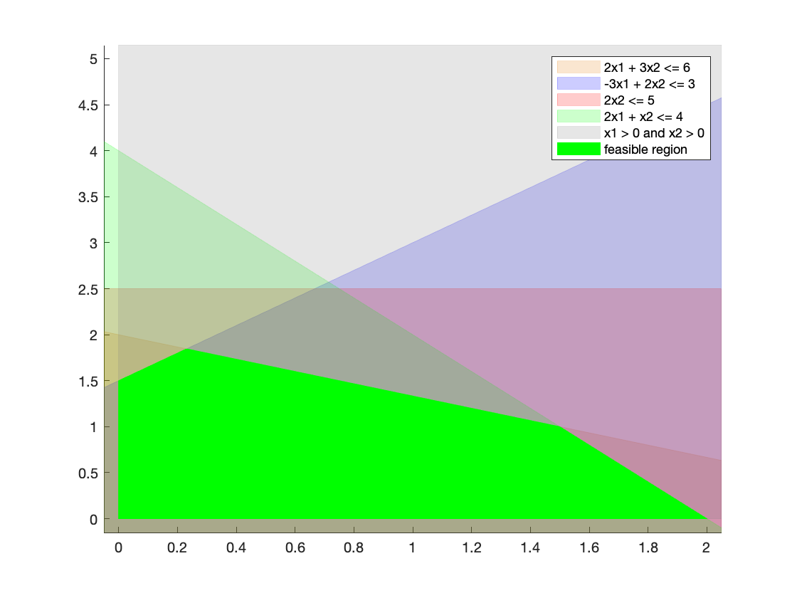
The resulting MATLAB plot of each constraint and of the feasible region is shown below:

$Plot of feasible region and constraints\label{fig:a}$

Exercise 2.2

According to Nocedal, a vector x is a basic feasible point if it is in the feasible region and if there exists a subset \beta of the index set 1, 2, \ldots, n such that:

\beta contains exactly m indices, where m is the number of rows of A;
For any i \notin \beta, x_i = 0, meaning the bound x_i \geq 0 can be inactive only if i \in \beta;
The m x m matrix B defined by B = [A_i]_{i \in \beta} (where A_i is the i-th column of A) is non-singular, i.e. all columns corresponding to the indices in \beta are linearly independent from each other.

The geometric interpretation of basic feasible points is that all of them are vertices of the polytope that bounds the feasible region. We will use this proven property to manually solve the constrained minimization problem presented in this section by aiding us with the graphical plot of the feasible region in figure \ref{fig:a}.

Exercise 2.3

Since the geometrical interpretation of the definition of basic feasible point states that these point are non-other than the vertices of the feasible region, we first look at the plot above and to these points (i.e. the vertices of the bright green non-trasparent region). Then, we look which constraint boundaries cross these edges, and we formulate an algebraic expression to find these points. In clockwise order, we have:

The lower-left point at the origin, given by the boundaries of the constraints x_1 \geq 0 and x_2 \geq 0:

$x^*_1 = \begin{bmatrix}0\\0\end{bmatrix

The top-left point, at the intersection of constraint boundaries x_1 \geq 0 and -3x_1 + 2x_2 \leq 3:

x_1 = 0 \;\;\; 2x_2 = 3 \Leftrightarrow x_2 = \frac32 \;\;\; x^*_2 =
\frac12 \cdot \begin{bmatrix}0\\3\end{bmatrix}$$

The top-center-left point at the intersection of constraint boundaries $-3x_1 + 2x_2 \leq 3$ and 2x_1 + 3x_2 \leq 6:

-3x_1 + 2x_2 + 3x_1 + \frac92 x_2 = \frac{13}{2} x_2 = 3 + 9 = 12
\Leftrightarrow x_2 = 12 \cdot \frac2{13} = \frac{24}{13}$$$$
-3x_1 + 2 \cdot \frac{24}{13} = 3 \Leftrightarrow x_1 = \frac{39 - 48}{13}
\cdot \frac{1}{-3} = \frac{3}{13} \;\;\; x^*_3 = \frac{1}{13} \cdot
\begin{bmatrix}3\\24\end{bmatrix}$$

The top-center-right point at the intersection of constraint boundaries $2x_1

3x_2 \leq 6$ and 2x_1 + x_2 \leq 4:

2x_1 + 3x_2 - 2x_1 - x_2 = 2x_2 = 6 - 4 = 2 \Leftrightarrow x_2 = 1 \;\;\;
2x_1 + 1 = 4 \Leftrightarrow x_1 = \frac32 \;\;\; x^*_4 = \frac12 \cdot
\begin{bmatrix}3\\2\end{bmatrix}$$

The right point at the intersection of 2x_1 + x_2 \leq 4 and $x_2 \geq 0$:

x_2 = 0 \;\;\; 2x_1 + 0 = 4 \Leftrightarrow x_1 = 2 \;\;\; x^*_5 =
\begin{bmatrix}2\\0\end{bmatrix}$$

Therefore, x^*_1 to x^*_5 are all of the basic feasible points for this constrained minimization problem.

We then compute the objective function value for each basic feasible point found, The smallest objective value will correspond with the constrained minimizer problem solution.


x^*_1 = \begin{bmatrix}0\\0\end{bmatrix} \;\;\; f(x^*_1) = 4 \cdot 0 + 3 \cdot 0 =
0$$$$
x^*_2 = \frac12 \cdot \begin{bmatrix}0\\3\end{bmatrix} \;\;\;
f(x^*_2) = 4 \cdot 0 + 3 \cdot \frac{3}{2} = \frac92$$$$
x^*_3 = \frac{1}{13} \cdot \begin{bmatrix}3\\24\end{bmatrix} \;\;\; f(x^*_3) = 4
\cdot \frac{3}{13} + 3 \cdot \frac{24}{13} = \frac{84}{13}$$$$
x^*_4 = \frac12 \cdot \begin{bmatrix}3\\2\end{bmatrix} \;\;\; f(x^*_4) = 4 \cdot
\frac32 + 3 \cdot 1 = 9$$$$
x^*_5 = \begin{bmatrix}2\\0\end{bmatrix} \;\;\; f(x^*_5) = 4 \cdot 2 + 1 \cdot 0
= 8$$

Therefore, $x^* = x^*_1 = \begin{bmatrix}0 & 0\end{bmatrix}^T$ is the global
constrained minimizer.

# Exercise 3

## Exercise 3.1

Yes, the problem can be solved with Uzawa's method since the problem can be
reformulated as a saddle point system. The KKT conditions of the problem can be
reformulated as a matrix-vector to vector equality in the following way:

$$\begin{bmatrix}G & -A^T\\A & 0 \end{bmatrix} \begin{bmatrix}
x^*\\\lambda^* \end{bmatrix} = \begin{bmatrix} -c\\b \end{bmatrix}.$$

If we then express the minimizer $x^*$ in terms of $x$, an approximation of it,
and $p$, a search step (i.e. $x^* = x + p$), we obtain the following system.

$$\begin{bmatrix}
G & A^T\\
A & 0
\end{bmatrix}
\begin{bmatrix}
-p\\
\lambda^*
\end{bmatrix} =
\begin{bmatrix}
g\\
h
\end{bmatrix}$$

This is the system the Uzawa method will solve. Therefore, we need to check
if the matrix:

$$K = \begin{bmatrix}G & A^T \\ A& 0\end{bmatrix} = \begin{bmatrix}
6  &   2  &  1  &  1  &  0 \\
2  &   5  &  2  &  0  &  1 \\
1  &   2  &  4  &  1  &  1 \\
1  &   0  &  1  &  0  &  0 \\
0  &   1  &  1  &  0  &  0 \\
\end{bmatrix}\text{ recalling the computed values of }A\text{ and }G\text{ from the
previous assignment}$$

Has non-zero positive and negative eigenvalues. We compute the eigenvalues of this
matrix with MATLAB, and we find:

$$\begin{bmatrix}
   -0.4818\\
   -0.2685\\
    2.6378\\
    4.3462\\
    8.7663\end{bmatrix}$$

Therefore, the system is indeed a saddle point system and it can be solved with
Uzawa's method.

## Exercise 3.2

The MATLAB code used to find the solution can be found under section 3.2 of the
`main.m` script. The solution is:

$$x=\begin{bmatrix}0.7692\\-2.2308\\2.2308\end{bmatrix} \;\;\; \lambda=
\begin{bmatrix}-10.3846\\2.1538\end{bmatrix}$$

10 KiB Raw Permalink Blame History