OM/Claudio_Maggioni_midterm/Claudio_Maggioni_midterm.md

---

title: Midterm -- Optimization Methods author: Claudio Maggioni header-includes:

• \usepackage{amsmath}
• \usepackage{hyperref}
• \usepackage[utf8]{inputenc}
• \usepackage[margin=2.5cm]{geometry}
• \usepackage[ruled,vlined]{algorithm2e}
• \usepackage{float}
• \floatplacement{figure}{H}

---

\maketitle

Exercise 1

Point 1

Question (a)

As already covered in the course, the gradient of a standard quadratic form at a point x_0 is equal to:

 \nabla f(x_0) = A x_0 - b 

Plugging in the definition of x_0 and knowing that $\nabla f(x_m) = A x_m - b = 0$ (according to the first necessary condition for a minimizer), we obtain:

\nabla f(x_0) = A (x_m + v) - b = A x_m + A v - b = b + \lambda v - b = \lambda v

Question (b)

The steepest descent method takes exactly one iteration to reach the exact minimizer x_m starting from the point x_0. This can be proven by first noticing that x_m is a point standing in the line that first descent direction would trace, which is equal to:

g(\alpha) = - \alpha \cdot \nabla f(x_0) = - \alpha \lambda v

For \alpha = \frac{1}{\lambda}, and plugging in the definition of $x_0 = x_m + v$, we would reach a new iterate x_1 equal to:

x_1 = x_0 - \alpha \lambda v = x_0 - v = x_m + v - v = x_m 

The only question that we need to answer now is why the SD algorithm would indeed choose \alpha = \frac{1}{\lambda}. To answer this, we recall that the SD algorithm chooses \alpha by solving a linear minimization option along the step direction. Since we know x_m is indeed the minimizer, f(x_m) would be obviously strictly less that any other f(x_1 = x_0 - \alpha \lambda v) with \alpha \neq \frac{1}{\lambda}.

Therefore, since x_1 = x_m, we have proven SD converges to the minimizer in one iteration.

Point 2

The right answer is choice (a), since the energy norm of the error indeed always decreases monotonically.

To prove that this is true, we first consider a way to express any iterate $x_k$ in function of the minimizer x_s and of the missing iterations:

x_k = x_s + \sum_{i=k}^{N} \alpha_i A^i p_0

This formula makes use of the fact that step directions in CG are all A-orthogonal with each other, so the k-th search direction p_k is equal to A^k p_0, where p_0 = -r_0 and r_0 is the first residual.

Given that definition of iterates, we're able to express the error after iteration k e_k in a similar fashion:

e_k = x_k - x_s = \sum_{i=k}^{N} \alpha_i A^i p_0

We then recall the definition of energy norm \|e_k\|_A:

\|e_k\|_A = \sqrt{\langle Ae_k, e_k \rangle}

We then want to show that \|e_k\|_A = \|x_k - x_s\|_A > \|e_{k+1}\|_A, which in turn is equivalent to claim that:

\langle Ae_k, e_k \rangle > \langle Ae_{k+1}, e_{k+1} \rangle

Knowing that the dot product is linear w.r.t. either of its arguments, we pull out the sum term related to the k-th step (i.e. the first term in the sum that makes up e_k) from both sides of \langle Ae_k, e_k \rangle, obtaining the following:

$$\langle Ae_{k+1}, e_{k+1} \rangle + \langle \alpha_k A^{k+1} p_0, e_k \rangle

• \langle Ae_{k+1},\alpha_k A^k p_0 \rangle > \langle Ae_{k+1}, e_{k+1} \rangle$$

which in turn is equivalent to claim that:

$$\langle \alpha_k A^{k+1} p_0, e_k \rangle

• \langle Ae_{k+1},\alpha_k A^k p_0 \rangle > 0$$

From this expression we can collect term \alpha_k thanks to linearity of the dot-product:

$$\alpha_k (\langle A^{k+1} p_0, e_k \rangle

• \langle Ae_{k+1}, A^k p_0 \rangle) > 0$$

and we can further "ignore" the \alpha_k term since we know that all $\alpha_i$s are positive by definition:

$$\langle A^{k+1} p_0, e_k \rangle

• \langle Ae_{k+1}, A^k p_0 \rangle > 0$$

Then, we convert the dot-products in their equivalent vector to vector product form, and we plug in the definitions of e_k and e_{k+1}:

$$p_0^T (A^{k+1})^T (\sum_{i=k}^{N} \alpha_i A^i p_0) + p_0^T (A^{k})^T (\sum_{i=k+1}^{N} \alpha_i A^i p_0) > 0$$

We then pull out the sum to cover all terms thanks to associativity of vector products:

$$\sum_{i=k}^N (p_0^T (A^{k+1})^T A^i p_0) \alpha_i+ \sum_{i=k+1}^N (p_0^T (A^{k})^T A^i p_0) \alpha_i > 0$$

We then, as before, can "ignore" all \alpha_i terms since we know by definition that they are all strictly positive. We then recalled that we assumed that A is symmetric, so A^T = A. In the end we have to show that these two inequalities are true:

p_0^T A^{k+1+i} p_0 > 0 \; \forall i \in [k,N]

p_0^T A^{k+i} p_0 > 0 \; \forall i \in [k+1,N]

To show these inequalities are indeed true, we recall that A is symmetric and positive definite. We then consider that if a matrix A is SPD, then A^i for any positive i is also SPD¹. Therefore, both inequalities are trivially true due to the definition of positive definite matrices.

Thanks to this we have indeed proven that the delta $|e_k|A - |e{k+1}|_A$ is indeed positive and thus as i increases the energy norm of the error monotonically decreases.

Question 2

Point 1

TBD

Point 2

The trust region algorithm is the following:

\begin{algorithm}[H] \SetAlgoLined Given \hat{\Delta} > 0, \Delta_0 \in (0,\hat{\Delta}), and $\eta \in [0, \frac14)$;

\For{$k = 0, 1, 2, \ldots$}{% Obtain p_k by using Cauchy or Dogleg method; $\rho_k \gets \frac{f(x_k) - f(x_k + p_k)}{m_k(0) - m_k(p_k)}$; \uIf{$\rho_k < \frac14$}{% $\Delta_{k+1} \gets \frac14 \Delta_k$; }\Else{% \uIf{\rho_k > \frac34 and $|\rho_k| = \Delta_k$}{% $\Delta_{k+1} \gets \min(2\Delta_k, \hat{\Delta})$; } \Else{% $\Delta_{k+1} \gets \Delta_k$; }} \uIf{$\rho_k > \eta$}{% $x_{k+1} \gets x_k + p_k$; } \Else{ $x_{k+1} \gets x_k$; } } \caption{Trust region method} \end{algorithm}

The Cauchy point algorithm is the following:

\begin{algorithm}[H] \SetAlgoLined Input B (quadratic term), g (linear term), $\Delta_k$; \uIf{$g^T B g \geq 0$}{% $\tau \gets 1$; }\Else{% $\tau \gets \min(\frac{|g|^3}{\Delta_k \cdot g^T B g}, 1)$; }

$p_k \gets -\tau \cdot \frac{\Delta_k}{|g|^2 \cdot g}$; \Return{$p_k$} \caption{Cauchy point} \end{algorithm}

Finally, the Dogleg method algorithm is the following:

\begin{algorithm}[H] \SetAlgoLined Input B (quadratic term), g (linear term), $\Delta_k$; $p_N \gets - B^{-1} g$;

\uIf{$\|p_N\| < \Delta_k$}{%
  $p_k \gets p_N$\;
}\Else{%
    $p_u = - \frac{g^T g}{g^T B g} g$\;

    \uIf{$\|p_u\| > \Delta_k$}{%
      compute $p_k$ with Cauchy point algorithm\;
    }\Else{%
        solve for $\tau$ the equality $\|p_u + \tau * (p_N - p_u)\|^2 =
        \Delta_k^2$\;
        $p_k \gets p_u + \tau \cdot (p_N - p_u)$\;
    }
}

\caption{Dogleg method} \end{algorithm}

Point 3

The trust region, dogleg and Cauchy point algorithms were implemented respectively in the files trust_region.m, dogleg.m, and cauchy.m.

Point 4

Taylor expansion

The Taylor expansion up the second order of the function is the following:

$$f(x_0, w) = f(x_0) + \langle\begin{bmatrix}48x^3 - 16xy + 2x - 2\2y - 8x^2 \end{bmatrix}, w\rangle + \frac12 \langle\begin{bmatrix}144x^2 -16y + 2 - 16 & -16 \ -16 & 2 \end{bmatrix}w, w\rangle$$

Minimization

The code used to minimize the function can be found in the MATLAB script main.m under section 2.4. The resulting minimizer (found in 10 iterations) is:

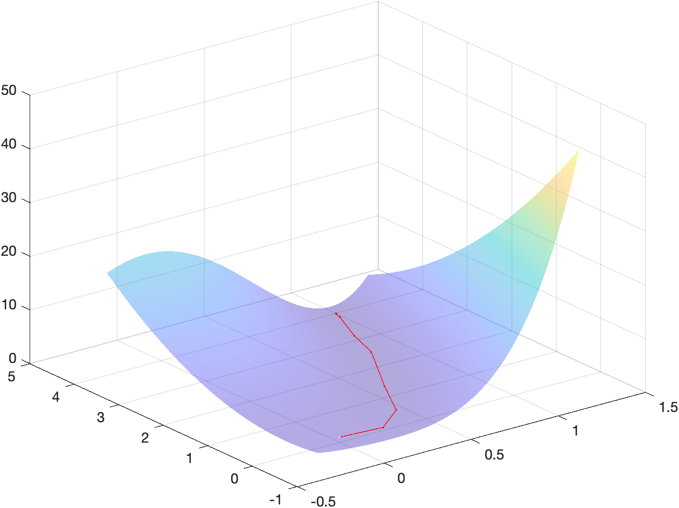
x_m = \begin{bmatrix}1\\4\end{bmatrix}

Energy landscape

The following figure shows a surf plot of the objective function overlayed with the iterates used to reach the minimizer:

The code used to generate such plot can be found in the MATLAB script main.m under section 2.4c.

Point 5

Minimization

The code used to minimize the function can be found in the MATLAB script main.m under section 2.5. The resulting minimizer (found in 25 iterations) is:

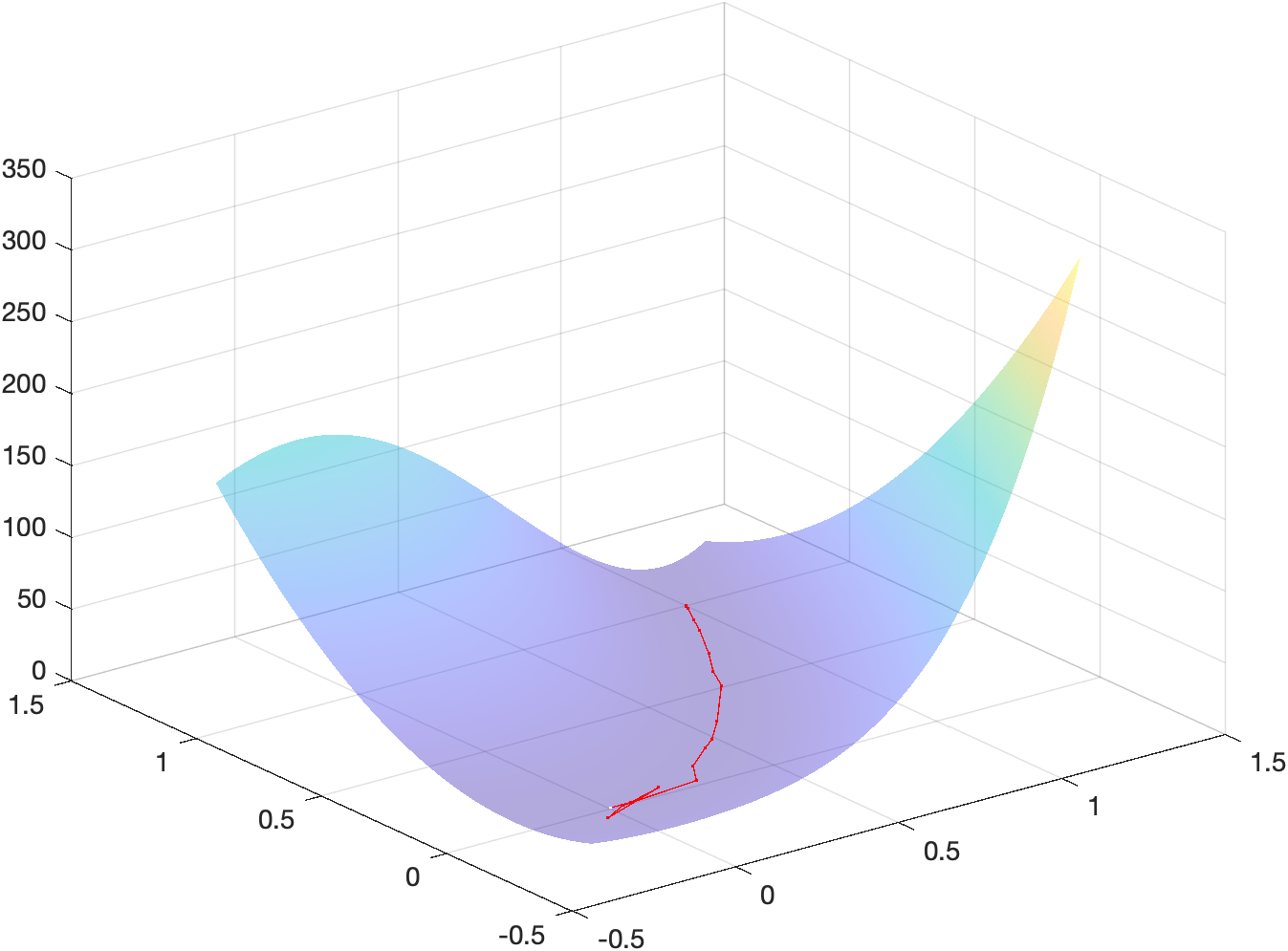
x_m = \begin{bmatrix}1\\5\end{bmatrix}

Energy landscape

The following figure shows a surf plot of the objective function overlayed with the iterates used to reach the minimizer:

The code used to generate such plot can be found in the MATLAB script main.m under section 2.5b.

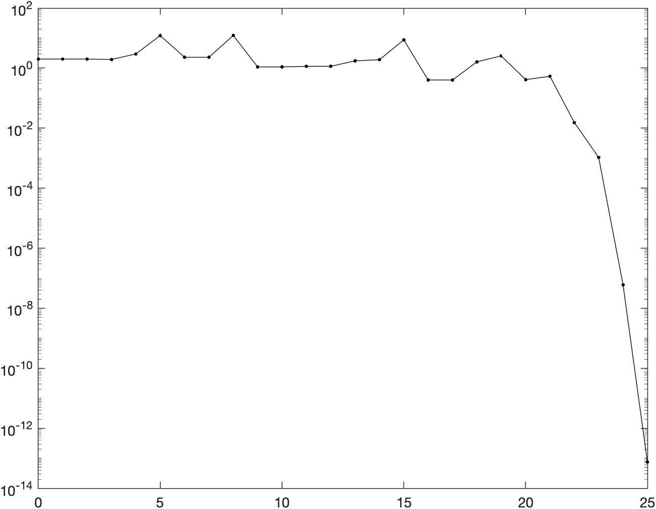
Gradient norms

The following figure shows the logarithm of the norm of the gradient w.r.t. iterations:

The code used to generate such plot can be found in the MATLAB script main.m under section 2.5c.

Comparing the behaviour shown above with the figures obtained in the previous assignment for the Newton method with backtracking and the gradient descent with backtracking, we notice that the trust-region method really behaves like a compromise between the two methods. First of all, we notice that TR converges in 25 iterations, almost double of the number of iterations of regular NM + backtracking. The actual behaviour of the curve is somewhat similar to the Netwon gradient norms curve w.r.t. to the presence of spikes, which however are less evident in the Trust region curve (probably due to Trust region method alternating quadratic steps with linear or almost linear steps while iterating). Finally, we notice that TR is the only method to have neighbouring iterations having the exact same norm: this is probably due to some proposed iterations steps not being validated by the acceptance criteria, which makes the method mot move for some iterations.

---

1. source: Wikipedia - Definite Matrix \to Properties $\to$ Multiplication ↩︎